
A REDERIVATION OF THE ELECTRICAL
TRANSMISSION LINE EQUATIONS USING NETWORK THEORY
SHOWS NEW TERMS THAT MATTER IN NEURAL TRANSMISSION.
M. Robert Showalter
ABSTRACT:
Some of the logic of neurophysiology depends on the
mathematical form of the passive electrical transmission equations that
apply to nerves. The electrical transmission line is modelled here by network
theory. The network model is inconsistent with the accepted transmission
equations,
dv/dx = -Ri -L di/dt and di/dx = -Gv -C dv/dt.
The network model shows an effective inductance that
depends on R and C. Results suggest that we have been underestimating effective
inductance in many neural passages by large factors.
It would be hard to pick equations in engineering physics that
are more useful, and that have been more extensively tested, than the electrical
line transmission equations.
dv/dx = -Ri -L di/dt (1)
di/dx = -Gv -C dv/dt (2)
where v = voltage
i = current x
= position along the line
R = resistance/length L=electromagnetic
inductance/length
G= membrane conductance/length
C=capacitance/length
R, L, G, and C are modelled as uniform along
the line. These equations are applied to different conductors. For example,
R may vary by a factor of 1015 from a wire to a neural
dendrite, with equations 1 and 2 applied in the same way to both the wire
and the dendrite. Totally satisfactory performance of equations 1 and 2
over the entirety of this huge range has been assumed.
Equations 1 and 2 were first applied to submerged telegraph
cables by Kelvin in 1855(1), and were combined
by Heaviside in 1887(2) to form the "Heaviside
equations" or "telegrapher's equations(3)"
that are fundamental to telephony and much of electrical and computer engineering.
Although Equations 1 and 2 both refer to flow of the same
charge carriers on the same line, dv/dx depends only on R
and L, and di/dx depends only on G and C.
This paper shows that both dv/dx and di/dx are functions
of all of the line properties R, L, G and C.
Some new terms are shown that are negligible for the usual transmission
lines of electrical engineering, but that can be dominant in the fine scale
dendrites and unmyelinated axons of neurons.
NEUROLOGICAL BACKGROUND:
The dendrites and axons of nerves are conducting lines. They are thought
to be without significant inductance. Many waveforms observed in dendrites
and axons look like reflection traces that occur on electrical transmission
lines, where inductance is important(4).
Three decades ago Lieberstein suggested that inductance was important in
neural transmission as well(5). However,
when the matter was investigated(6) (7),
no plausible source of the inductance required was found. Wilfred Rall
expressed the conclusion drawn as follows(8).
The "cable equation" Rall refers to is equation 1 with L=0, combined
with equation 2.
"Comment: Cable Versus Wave Equations
" The cable equation, heat conduction equation, and diffusion
equation are all partial differential equations of the same parabolic type.
Such equations, and their solutions, differ significantly from those of
the elliptical type (e.g. Laplace's equation or potential theory) and from
those of hyperbolic type (e.g. electromagnetic wave equation.) When electromagnetic
inductance is added to a telegraph cable or transmission line, the partial
differential equation gains a term that is proportional to
and this changes the equation from the parabolic type to the hyperbolic
type; engineers have long known that this can enhance telegraph signal
propagation. However important this is for engineering, a recent attempt
to account for nerve propagation as a wave solution to such a differential
equation can be dismissed for two important reasons: not only did this
involve a misunderstanding of the nonlinear membrane properties elucidated
by Hodgkin and Huxley, it tacitly assumes an amount of electromagnetic
inductance that far exceeds the negligible amount present in nerve."
This paper shows an effective inductance that
is inversely proportional to the cube of neural passage diameter. At the
scale of most neurons, this effective inductance appears to be > 1011
times larger than the inductance that Rall considered.
Implications of this increased inductance for neural science and
neural medicine, and evidence for it, are discussed in a companion paper(9).
With the increased inductance, unresolved issues in neural transmission
and neural time response can be explained. Ubiquitous but now unexplained
effects, phenomenologically similar to resonance, can be explained in resonant
terms.
TRANSMISSION LINES AND KIRCHHOFF'S LAWS:
Fig 1 shows a neural conductor (transmission line). A tubular membrane is filled with and surrounded by an ionic fluid. The fluid inside the tube carries current (and signal) and has resistance R and electromagnetic inductance L per unit length. The outer fluid is grounded. In convenient units, the membrane separating the inner and outer ionic fluids has capacitance c in farads/cm2 and conductance g in mhos/cm2. The fluid has a
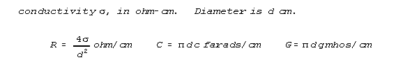
Fig 1 shows an arbitrarily chosen length beta, picked from other
indistinguishable length sectors illustrated. The circumferential lines
that separate the sectors shown are analytic constructs, like grid lines.
There is nothing special or physically causal about the beginning and endpoints
for the length beta that happens to be chosen for analysis.
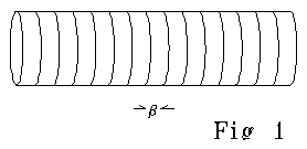
The tube of Fig 1 is modelled as a pair of mathematical lines that
are homogeneous, continuous, differentiable, and indefinitely long. The
grounded external fluid is modelled as a 0 resistance, 0 inductance line.
The inner, signal carrying line has uniformly distributed resistance R
and inductance L, uniformly distributed capacitance C to the ground line,
and uniformly distributed current leakage G to the ground line. This is
a continuum MATHEMATICAL model. The scale beta could be 10-5,
10-50, or 10-500 meters long, and the logic and geometry
of the model would stay the same.
This homogeneous and differentiable line pair is typically visualized
as a series of arbitrarily small 4-pole elements connected end-for-end
as shown in Fig 2, with a single 4-pole element set out in enlarged detail
in Fig 2a. Fig 2a shows symbols for the discrete elements of R, L, G and
C.
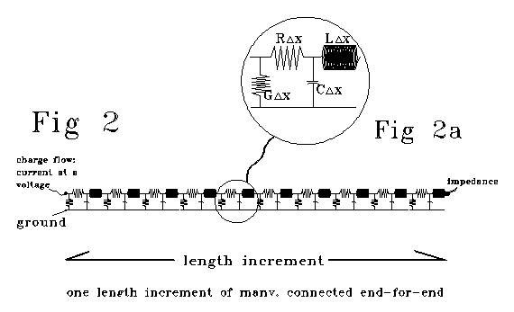
Fig 2 is shown as one "length increment" long. That "length
increment" might be a millimeter, or 10-50 meters long
- the representation that is Fig 2 would look the same. We will show that
we CANNOT derive equations 1 and 2 from an "almost differentially
short" Fig 2. We will also show that an "almost differentially
short" model like Fig 2, but consisting of 20, 80, 400, or n RLGC
elements rather than the 10 that Fig 2, will yield results that depend
on choice of n.
Let's call incremental voltage and current as functions of position
x and time t
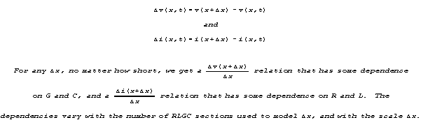
KIRCHHOFF'S LAWS AND THE FUNCTIONAL DEPENDENCIES OF dv/dx AND di/dx:
Fig 2 has the form of a ladder filter, a common kind of bandpass
filter(10). Let's consider the RLGC network
of Fig 2 according to network theory, following Skilling's encyclopedia
article(11). The elements of the network
are the resistors, inductors and capacitors, corresponding to the symbols
R, L, G, and C. (R corresponds to series resistance; G is the reciprocal
of shunt resistance.) Nodes connect three or more elements together. Branches
connect two nodes, and may include one or more elements in series. A loop,
or circuit, is a single closed path for current. A mesh is a loop with
no interior branch.
Charge is conserved. This fact applied to nodes is Kirchhoff's current
law: the sum of currents entering a node is 0.
![]()
Current equations of this form can be written for each of the N nodes
in a circuit. N-1 of these equations will be independent. Voltage is a
property, and hence path independent. This fact applied to loops is Kirchhoff's
voltage law. The sum of voltage changes around a loop (from a point back
to that point) is zero.
![]()
Voltage equations of this form can be written for each of the loops
in a circuit. Not all of these equations are independent.
The number of independent loops, Llp can be computed from
E = N + Llp
where N and E are the number of nodes and elements. For a planar,
fully connected network like Fig 2, the number of independent loops is
the same as the number of meshes.
Fig 2 has 10 RLGC elements, 20 nodes and 20 meshes. For m RLGC elements
placed end-for-end, there will be 2m nodes and 2m meshes. E, the number
of elements, is 4m. B, the number of branches, is 6m.
Details of setup and solution of the equations corresponding to loops
and nodes are set out in Skilling(12).
The essential point here is that solving for the currents and voltages
of a network such as the one of Fig 2 can be reduced to either
solving Llp linear loop equations, solving currents from
which voltages follow directly or
solving N linear node equations, solving voltages from which currents
follow directly.
We can see some things about the network of Fig. 2 by inspection. In Fig 2, every loop has both a series and a shunt element, and every node has both a series and a shunt element. Whether circuit analysis were done using node equations or loop equations, voltage and current would be determined by systems of equations consisting only of equations with both series and shunt elements. This means that, in contrast to equation 1, the full dv/dx relation must have some dependence on G and C. In contrast to equation 2, the full di/dx relation must have some dependence on R and L.
Calculation shows what these dependencies are. Software for these
calculations is widely available. The de facto standard for analog circuit
simulation is SPICE from the U. of C. at Berkeley, and its commercial embodiments(13)
(14) (15).
Typical design of complicated circuits is now a dialog between SPICE-derived
simulation and experimental checking, and over time this dialog has checked
and validated SPICE. Although SPICE does much else, the heart of SPICE
consists of routines that solve circuit network equations consisting of
passive elements like those of Fig 2. The network equations are derived
from Kirchhoff's laws and the laws for R, L, and C. The equations are then
solved by linear algebra, according to the standard patterns set out above.
A powerful demo program of PSpice, a commercial version of SPICE, is free.
The results below are were derived using this demo. The demo PSpice program,
the input programs that generated that graphs shown below, and the computer
programs that yielded the input instructions that generated the graphs,
are made available by ftp(16). We are using
PSpice here to do Kirchhoff network models of a transmission line. PSpice
contains separate transmission line subroutines, based on equations 1 and
2, that are computationally much faster than the Kirchhoff models set out
here. These subroutines embody assumptions that the Kirchhoff model does
make, that we are investigating here.
Let Fig 1 refer to a section of neuronal line. We can model a set
length of that line using a RGLC-RGLC-RGLC ... network such as Fig 2. For
the same length, we can use a modelling network with different numbers
of evenly spaced and matched RGLC sections, adjusting the values of the
individual R, G, L and C elements so that they add up to the R, G, L and
C over the modelled length . Sometimes we may simplify the model, and deal
with RC sections with G and L set to 0, or model a series of RG sections
with C and L set to 0. With the simpler RC and RG models we can compute
more sections in series than we can with RGLC networks.
Consider Fig 1 as a neural dendrite of .1 micron diameter. We set
membrane capacitance at 10-6 farad/cm2. The passage
is filled with an ionic fluid with a resistivity, , of 110 ohm-cm. We choose
the electromagnetic inductance of a single line, which is no function of
diameter.) Membrane resistance, which occurs by opening and closing of
populations of membrane channels, can vary by many orders of magnitude
from time to time. Line properties are
R =1.40x10¹² ohm/cm L =5x10⁻⁹ henries/cm
C =3.16x10⁻⁵ microfarad/cm G
= variable
We'll set L = 0, judging it to be negligible in comparison with R.
The case where G is also 0, so that the dendrite is an R-C system, will
be treated first.
Graphs 31-34 show calculations for this R-C dendrite, corresponding
to Fig 1, for a length of 10-5 cm (.1 micron.) The dendrite
is modelled as the "ladder filter" of Fig 2, with 20, 40, and
80 RC loops in series. AC input current is 1 nanoamp swept from 1 to 40,000
Hz. Output impedance in the models is negligible (the end of the line dumps
to ground through .0001 line resistance) so that voltage varies about linearly
from one end of these lines to the other. Voltage drops across resistors
are plotted as resistor voltage drop divided by resistor modelling length,
x (x = .05µ, .025µ, and .0125µ for the 20, 40, and 80
loop cases.) v/x in these models depends on capacitance as well as resistance.
Voltage drop across the resistors changes because current storage in membrane
capacitance causes current to change along the line.
Graph 3-1 is for 20 RC groups. Curves are plotted for every 2d resistor.
Graph 3-2 models 40 RC groups. Curves are plotted for every 4th resistor.
Graph 3-3 models 80 RC groups. Curves are plotted for every 8th resistor.
Graph 3-4 is also for 80 groups, with C = 0.
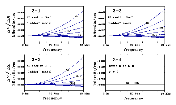
Graphs 31, 32, and 33 look much alike. Graph 34 shows that
gradients corresponding to dv/dx do not change from one resistor to the next, when capacitance is 0. Although these models are for a line length of 10-5 cm, similar effects are calculated for shorter lengths also. These PSpice calculations on this ladder model imply that no matter how short a delta x we choose, there will be a finite capacitance effect on values of [delta v(x,t)]/(delta x). We may investigate this dependence in more detail. We've set L=0, so Equation 1 reduces to dv/dx = -Ri. In finite increment form, this integrates over an interval delta x as
![]()
The residual of voltage not explained by Ohm's law is

the calculated voltage difference over an interval minus the voltage
predicted by Ohm's law over that interval, using the average current over
the interval. An "effective inductance" is calculated, as shown
in graphs 4a, 4b, 4c, and 4d.
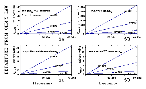
The "effective inductance" per unit length shown in Figs
4A-4D works out to be proportional to R2C/4 (length2).
The relation of the models of Figs 4B, 4C, and 4D to the model of Fig 4A
illustrate this. Each of these models changes one value of the Fig 4A model,
leaving others the same. Comparing output voltages, 4B/4A shows an effective
inductance per unit length proportional to length2; 4C/4A shows
proportionality to capacitance; and 4D/4A shows proportionality to the
square of resistance. All the points on all the lines of Figs 4A-4C seem
to be the same within 1 part per 10,000, except for the factors of 10 shown.
The lines shown are straight, showing proportionality to di/dt (the operational
definition of inductance.)
Fig 5 corresponds to Fig 4A, and shows that the calculated effective inductance term is a small residual compared to system voltages in this calculation.
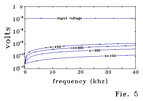
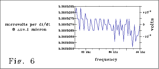
Fig. 6 also corresponds to the case of Fig 4a, and shows the 400
loop model line of 4A divided by di/dt for frequencies from 15-40 kzh.
[ di/dt=10-9 amps*(2 pi frequency) amps/sec]. The vertical axis
plots 5.0585286 millivolts +/- .2 nanovolts. Fig 6 illustrates the good
but still limited quality of the PSpice model numerics, the close proportionality
of the curve to di/dt, and a value of effective inductance that is .9850
[(R2C)/12 (delta x)2], a value close to R2C/12
(length2).
Figs 4A-4D were plotted for models with 40, 20 and 10 times more
sections than the 10 section length illustrated in Fig 2 for a computational
reason. Fig 7 illustrates calculated results analogous to those of Fig
4A, with the same .1 micron length, same capacitance, and same conductance,
with the length divided into 400 and smaller numbers of sections. Calculated
values depend strongly on the number of sections. Data bars in Fig. 7 are
fit to a polynomial curve for interpolation. The behavior shown in Fig
7 may merit the term "insidious." The effect occurs in proportion
to crossproducts (such as R2C) that may vary over many tens
of orders of magnitude from case to case. For a conventional wire, this
product might be of the order of 10-80 or less, too small to
attend to (and too small for numerics to catch.) Even when the crossproduct
magnitude is large, the effect may be missed if only a few sections are
calculated. However, the effect is systematic and nonlinear, and it builds
up. I have been limited to about 400 RC sections, and have only tested
ten sets of values for R and C, but I now suspect that calculations with
more sections must stabilize, subject to numerical build-up errors, near
the limit suggested by Fig. 7.
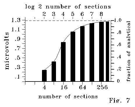
Fig 7 shows that the residual shown in Figs 4A-4C requires a fine
grid scale of calculation to approach equilibrium. However, at courser
scales, far from equilibrium, the functional dependence of the relation
on the variables is the same. For instance, curves like those of Figs 4A-4c
were calculated with 80, 60, 40, and 20 sections (rather than 400, 300,
200 and 100 sections of the Fig 4 series.) Values were different in the
proportion shown by Fig 7, and each of the curves in a single calculated
case departed noticeably from a 803:603:403:203
relation, with departures following the proportions shown in Fig 7. Even
so, comparing these courser cases, at a length ratio of 10:1 produced a
calculated voltage deviation from Ohm's law in an 1000:1 ratio. This ratio
held to .1% or better for all the curves compared. Similar comparisons
showed dependence on R2 and C to similar precision, according
to the logic shown in the Fig 4 series.
Figs 4A and 4B show that the integrated inductive effect over a length
goes as length3, so that "effective inductance" per
unit length goes as the square of length. Real measurements measure over
intervals, never at points. Here, the effective inductance depends radically
on the scale at which it is "effectively measured," an important
departure from the behavior of measurable quantities in the world.
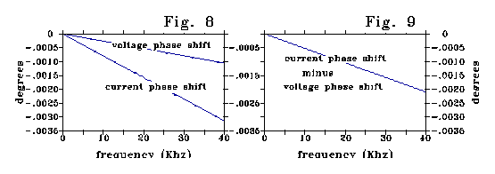
Inductance generates a LAG between current and voltage. The RC ladder
model shows such an i-v phase shift for the scale of small neural dendrites.
Fig 8 plots voltage and current phase, and Fig 9 the phase difference between
them. The value of effective inductance calculated from this phase shift
matches the inductance calculated as a deviation from Ohm's law to four
significant figures.
For the .1 micron diameter, .1 micron length of Fig 4A, the phase
shift and voltage effect corresponds to an inductance per unit length of
507 henries/cm from Fig 4a - a factor of 1011 larger than the
electromagnetic inductance (5x10⁻⁹ henries/cm) calculated for
the dendrite. Evaluated over a 1 micron length, the effective inductance
per unit length is 100 times larger still.
G DEPENDENCES:
So far we've shown that equation 1 depends on C. Equation 1 also
depends on G. The dependence, as a deviation from Ohm's law over an interval
delta x, depends on both voltage and current. Using the same procedures
shown above for the RC line, and assuming that coefficients close to 1
represent 1, the voltage dependency of (delta v)/(delta x) is

The current dependency is

Kirchhoff's law models of equation 2 after the pattern of Fig 2 indicate
that di/dx = -Gv -C dv/dt must also be incomplete. The i(x,t)/x relation
changes with R and L. Because electromagnetic L seems negligible in neurons,
we investigate only the R dependence. Using the same techniques illustrated
in Figs 3 and Figs 4, we find the i/x relation below.

SUMMARY OF RESULTS:
Compared to the finite increment form of equation 1

and the finite increment form of equation 2

our Kirchhoff network model estimates equations 1K and 2K:
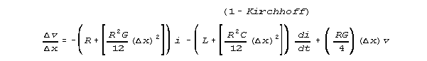
and

CONCLUSION:
The standard equations 1 and 2 convert directly to differential equations,
but the numerically derived Kirchhoff equations do not convert directly
to differential equations. The subexpressions

may appear infinitessimal by the usages of calculus. However, these
numerically derived subexpressions are definite results of a linear algebraic
process. We cannot dismiss these subexpressions by a limiting argument.
Setting delta x at zero, the terms in delta x will be zero, too. But we
know from our network model that if delta x is then evaluated at larger
and larger values, the subexpression will not stay "infinitessimal"
but will grow. What are we to make of these Kirchhoff model derived correllations,
with these awkward subexpressions? For many purposes in transmission modelling,
we'll need differential equations analogous to (1) and (2). We therefore
wish to argue for a particular differential equation, based on our knowledge
of the Kirchhoff correllations 1 and 2.
Let's take an approach that appeals to data. If we could use a specific
scaling delta x, and algebraically simplify the subexpressions

into expressions that did not depend on any particular value of delta
x, we'd then have

and

These equations could be converted directly into differential equations
useful for modelling neural transmission. More generally, reasoning from
our Kirchhoff model results, we could assume equations of the form of these
equations, and try to fit them to data.
I do this in a companion paper9. The ki's that
match biological data appear to be about 1. There appears to be an effective
inductance in neural transmission that can be, for neural diameters, between
1012 and 1021 times greater than the inductance that
is now assumed.
NOTES:
1. William Thomson, Lord Kelvin Proceedings of the Royal Society May 1855. Reprinted as article LXXXIII in Mathematical and Physical Papers by Sir William Thomson, Cambridge Press, 1884.
2. O. Heaviside ELECTRICAL PAPERS V.II Section XXXII 76-81 Chelsea Publishing Company 1970.
3. S. Rosenstark TRANSMISSION LINES IN COMPUTER ENGINEERING p 5 McGraw Hill, 1994.
4. David T. Stephenson "Transmission Lines" Fig 2. McGraw-Hill Encyclopedia of Science and Technology, 7th ed 1992.
5. Lieberstein, H.M. Mathematical Biosciences 1, 45-69 (1967).
6. S. Kaplan and D. Trujillo Mathematical Biosciences, 7 , 379-404, 1970.
7. A.C. Scott Mathematical Biosciences 11: 277-290, 1971.
8. W. Rall HANDBOOK OF PHYSIOLOGY: THE NERVOUS SYSTEM ( Kandell, E.R., ed) p. 60. (American Physiological Society Bethesda, Md. 1977.)
9. M.R. Showalter "New terms in the transmission line equations derived using network theory fit biological data" simultaneous submission
10. DeVerl S. Humpherys THE ANALYSIS, DESIGN, AND SYNTHESIS OF ELECTRICAL FILTERS Prentice Hall, Englewood Cliffs, N.J. 1970.
11. Hugh H. Skilling "Network theory" in McGraw Hill Encyclopedia of Science and Technology 5th ed. New York, 1982.
12. Skilling, op. cit. and H.H. Skilling ELECTRIC NETWORKS Wiley, New York, 1974.
13. L.W. Nagel SPICE2: A computer program to simulate semiconductor circuits, Memorandum No. m530 (May 1975) The Regents of the University of California, Berkeley, Ca.
14. W.J. McCalla FUNDAMENTALS OF COMPUTER-AIDED CIRCUIT SIMULATION Kluwer Academic 1988.
15. Paul W. Tuinenga SPICE: A guide to circuit simulation and analysis using PSpice 2nd ed. Prentice Hall, Englewood Cliffs, N.J. 1992.